If you need to filter a column in Google sheets for multiple values. The easiest way is to apply some conditional formatting to highlight the affected cells.
These are the steps needed.
- Disable all filters on the sheet.
- Select the column you want to apply the matching to.
- Right click and select conditional formatting
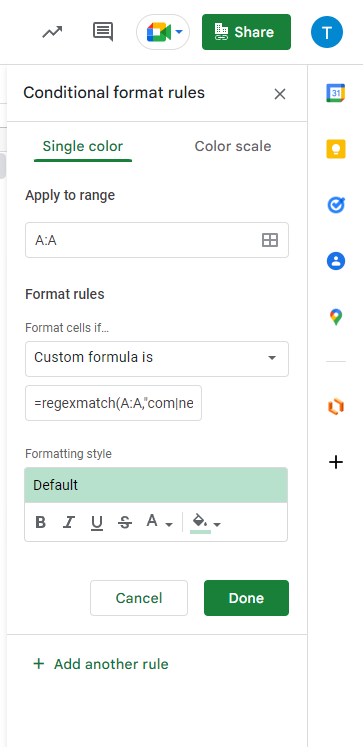
- Apply to Range – make sure this is the area you want matching to occur
- Format Rules – select custom formula is
- Enter this formula – =regexmatch(A:A,”com|net|org|ca|us”)
- Select the formatting style – Default is green
- Done
- The cells that match the text should now be highlighted. You can use the filter to include or exclude those cells.
=regexmatch(A:A,”com|net|org|ca|us”)
A:A is the range
com is a value to match
| is a separator
Remove | and words not needed to match